
Prepared in cooperation with the U.S. Army Corps of Engineers, Kansas City District
ONLINE ONLY
Appendix 1. Georeferenced locations within AOC 3 (table 1-1), AOC 7 (table...
Appendix 2-1. Graphs representing the total percent frequency of occurrence...
Appendix 2-2. Graphs representing the total percent frequency of occurrence...
Appendix 2-3. Graphs representing the total percent frequency of occurrence...
Appendix 3. Environmental noise tests on A, April 21, 2004 and B, April 22,...
Appendix 4. Table showing coordinates of zone boundaries.
Figure 1. Location of the areas of concern (AOCs), former Tyson Valley Powd...
Figure 2a. Results of the electromagnetic and magnetic survey at AOC 3 showi...
Figure 3. Site map of AOC 3 showing anomalous zones.
Figure 4. Photographs of surface metal at AOC 3 including exposures of smal...
Figure 5a. Results of the electromagnetic survey at AOC 7 (A and B) and AOC ...
Figure 6a. Results of the electromagnetic and magnetic survey at AOC 7 show...
Figure 7. A1 and A2, photographs of surficial metal in AOC 7 looking south ...
Figure 8. Site map of AOC 7 showing anomalous zones.
Figure 9a. Results of the electromagnetic and magnetic survey at AOC 10 show...
Figure 10. Photographs of surficial scrap metal in AOC 10 between mark -80,...
Figure 11. Site map of AOC 10 showing anomalous zones.
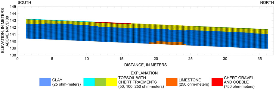
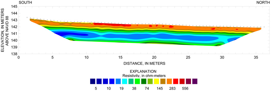
Figure 12. Field data of survey line 1 in AOC 3. Sections showing inverted...
Figure 13. Field data of survey line 2 in AOC 3. Sections showing A, invert...
Figure 14. Field data of survey line 3 in AOC 3. Sections showing A, invert...
Figure 15. Field data of survey line 4 in AOC 7. Sections showing A, invert...
Figure 16. Field data of survey line 5 in AOC 7. Sections showing A, inver...
Figure 17. Survey line 1, AOC 3. Sections showing A, forward model, and inv...
Figure 18. Survey line 2, AOC 3. Sections showing A, forward model, and B, ...
Figure 19. Survey line 3, AOC 3. Sections showing A, forward model, and B, ...
Figure 20. Survey line 4, AOC 7. Sections showing A, forward model, and B, ...
Figure 21. Survey line 5, AOC 7. Sections showing A, forward model, and B, ...
Figure 22. Section showing interpretation of inverted field resistivity, in...
Figure 23. Section showing interpretation of inverted field resistivity, in...
Figure 24. Section showing interpretation of inverted field resistivity, in...
Figure 25. Section showing interpretation of inverted field resistivity, in...
Figure 26. Section showing interpretation of inverted field resistivity, in...
Figure 27. Photographs taken during excavation activities at A, AOC 3, show...
Table 1-1. Georeferenced locations within AOC 3.
Table 1-2. Georeferenced locations within AOC 7.
Table 1-3. Georeferenced locations within AOC10.
1 U.S. Geological Survey, Lincoln, Nebraska.
2 U.S. Geological Survey, Lakewood, Colorado.
3 U.S. Army Corps of Engineers, Kansas City District, Kansas City, Missouri.
| Multiply | By | To obtain |
|---|---|---|
| Length | ||
| meter (m) | 3.281 | foot (ft) |
| kilometer (km) | 0.6214 | mile (mi) |
| Area | ||
| hectare (ha) | 0.003861 | square mile (mi2) |
| Volume | ||
| liter (L) | 2.113 | pint (pt) |
| liter (L) | 1.057 | quart (qt) |
| cubic meter (m3) | 0.2642 | gallon (gal) |
| liter (L) | 0.9464 | cubic inch (in3) |
Vertical coordinate information is referenced to the North American Vertical Datum of 1988 (NAVD 88).
Horizontal coordinate information is referenced to the North American Datum of 1983 (NAD 83).
Elevation, as used in this report, refers to distance above the vertical datum.
| 2D-DC | resistivity two-dimensional direct-current resistivity |
|---|---|
| AOC | area of concern |
| EM | electromagnetic |
| EMI | electromagnetic induction |
| Hz | hertz |
| kHz | kilohertz |
| m | meter |
| mS/m | millisiemens per meter |
| mV/V | millivolt per volt |
| nT | nanotesla |
| ppm | parts per million |
| RTK GPS | real-time kinematic global positioning system time-domain |
| IP | time-domain induced polarization |
| TRC | Tyson Research Center |
| TVPF | Tyson Valley Powder Farm |
The former Tyson Valley Powder Farm near Eureka, Missouri, was used primarily as a storage facility for the production of small arms ammunition during 1941–47 and 1951–61. A secondary use of the site was for munitions testing and disposal. Surface exposures of small arms waste, characterized by brass shell casings and fragments, as well as other miscellaneous scrap metal are remnants of disposal practices that took place during U.S. Army operation and can be found throughout the site. Little historical information exists describing disposal practices, and more debris is believed to be buried in the subsurface. The U.S. Army Corps of Engineers has identified several areas of concern throughout the former Tyson Valley Powder Farm. A surface-geophysical investigation was performed by the U.S. Geological Survey, in cooperation with the U.S. Army Corps of Engineers, to evaluate the areal and vertical extent of metallic debris in the subsurface within three of these areas of concern.
Electromagnetic and magnetic methods were used to locate anomalies indicating relatively large concentrations of buried metallic debris within the selected areas of concern. Maps were created identifying twelve anomalous zones in the three areas of concern, and three of these zones were selected for further investigation. The extent and depth of the anomalies within these zones were explored using two-dimensional direct-current resistivity methods. Resistivity and time-domain induced polarization data were compared to the anomalous locations of the electromagnetic and magnetic surveys.
The geophysical methods selected for this study were useful in determining the areal and vertical extent of metallic waste within the former Tyson Valley Powder Farm. However, electromagnetic and magnetic methods were not able to differentiate magnetic scrap metal from non-magnetic metallic small arms waste, most likely due to the small size and scattered distribution of the small arms waste, in addition to the mixing of both types of debris in the subsurface.
Electromagnetic and magnetic data showed some zones of concentrated anomalies, while there was a general scattering of small anomalies throughout the site. Inverted resistivity sections, as well as induced polarization sections, showed the debris to have a maximum depth of approximately 1 to 2 meters below the surface.
The former Tyson Valley Powder Farm (TVPF) was owned and operated by the U.S. Army from 1941–47, and again from 1951–61. The former TVPF was used primarily as a storage facility for the production of small arms ammunition, although munitions testing and disposal took place on the site as well (Kring and Bailey, 2001). During U.S. Army operation, shell casings, munitions, munitions components, storage drums, and miscellaneous metallic materials were disposed of throughout the property. During the second phase of operation in the 1950's, the site also was used for the storage of artillery rounds and chemicals used in tracers and incendiary devices (Francis Zigmund and C.R. Colbert, U.S. Army Corps of Engineers, oral commun., 2004). However, little historical information exists describing disposal practices during U.S. Army operation.
A remedial investigation (RI) conducted by the U.S. Army Corps of Engineers (USACE) has identified several areas of concern (AOCs) for potential soil and water contamination within the former TVPF. Soil samples from AOCs 3, 7, and 10 revealed relatively elevated concentrations of various trace elements, including mercury and arsenic. Surface exposures of shell casings were present in AOCs 3 and 7, as well as storage drums and miscellaneous scrap metal in AOC 10; however, the spatial extent and depth of these items in the subsurface were unknown. Surface geophysical techniques provide a quick, inexpensive, and non-intrusive means of collecting data in the subsurface environment. By applying electromagnetic (EM), magnetic, two-dimensional direct-current resistivity (2D-DC resistivity), and time-domain induced polarization (time-domain IP) methods, the extent and depth of anomalies in the signals potentially resulting from buried metallic objects can be characterized. The U.S. Geological Survey (USGS), in cooperation with the USACE, investigated AOC 3, AOC 7, and AOC 10 for subsurface metallic debris using surface geophysical methods. The results of this study will aid the USACE, Kansas City District, in performing removal of metallic debris under the Defense Environmental Restoration Program and in identifying potential locations for ground-water monitoring wells.
This report describes the results of EM and magnetic geophysical surveys used in AOCs 3, 7, and 10 with the purpose of defining the areal extent of buried small arms ammunition waste and scrap metal. Selected anomalies identified by the EM and magnetic surveys were characterized vertically with 2D-DC resistivity and time-domain IP methods. The results of excavation activities are also presented, in which some selected anomalies were excavated to assess the accuracy of the geophysical surveys.
The former TVPF site is in St. Louis County, Missouri. The site is approximately 32 kilometers southwest of the City of St. Louis and 5 kilometers northeast of the City of Eureka. The site occupies approximately 1,060 hectares and is divided into three areas: Tyson Research Center (TRC), Lone Elk County Park, and West Tyson County Park (Kring and Bailey, 2001) (fig. 1).
AOCs 3, 7, and 10 lie within the TRC property, which is currently (2004) owned and operated by Washington University at St. Louis as a biological field station. The property is approximately 796 hectares in size and is bounded on the north by the Burlington Northern Railroad and the Meramec River. Interstate 44 is the southern property boundary. The east and west boundaries of the TRC are Lone Elk Park and West Tyson County Park, respectively (Ellis Environmental Group, 2003) (fig. 1).
AOC 3, the Popping Kettle area, covers 0.26 hectare. It is near the northeasternmost boundary of the TRC property, and is situated on the steeply sloping forested hillside east of the Popping Kettle building. A small, somewhat incised ephemeral stream flows through the site northward toward the Meramec River. This area was primarily used for the demilitarization of off-specification and chemically treated .30- and .50-caliber ammunition by use of large, heated kettles. Molten primers and anvils plus an inorganic slag were placed in 55-gallon drums and/or dumped on the ground at AOC 3 (Francis Zigmund and C.R. Colbert, U.S. Army Corps of Engineers, oral commun., 2004). Numerous shell casings and rusty drums, both partially exposed at the surface and buried, have been found along and within the banks of the stream channel. All of the drums on the surface containing slag, some of the small arms waste in the upper part of the creek bed, and slag piles adjacent to the Popping Kettle building were removed during a Time Critical Removal Action (TCRA) performed by Anlab Environmental in November 1998 (U.S. Army Corps of Engineers, 2001). Small arms waste can still be found in the stream channel.
AOC 7, the Low Water Bridge Open Dump Site, is near the north edge of the TRC property. AOC 10 is immediately north of AOC 7 and forms its northern boundary. The south and east boundaries of AOC 7 are bordered by a gravel road. Tyson Hollow Creek, an intermittent stream, defines the western boundary. Although the majority of the site is covered by deciduous forest, the southeastern part of AOC 7 is open and grassy. This site was used as a disposal area for incinerated .30- and .50-caliber small arms waste (HydroGeoLogic, 1999).
AOC 10, the Scrap Metal Open Dump Site, is in a heavily wooded area directly north of AOC 7 and is on a sloping hillside. The eastern part of the site is an open field that ends at a gravel road. AOC 10 is bounded on the north by a small, unnamed intermittent stream and to the west by Tyson Hollow Creek. Angle iron, metal cable, metal drum remnants, and construction debris are exposed throughout the site and are concentrated near Tyson Hollow Creek.
Relatively elevated concentrations of mercury were detected in two shell casings and one composite soil sample collected from the streambed at AOC 3 in 1996 by the USACE (Ellis Environmental Group, 2003). RIs were conducted to delineate the nature and extent of contamination within the TRC. During the Phase I and II RIs, performed by HydroGeoLogic, Inc., soil samples were collected at multiple locations. Sample analytes included volatile organic compounds (VOCs), semivolatile organic compounds (SVOCs), target analyte list (TAL) contaminants, explosives and cyanide. Antimony, arsenic, barium, copper, lead, and zinc were detected in samples collected from the slag disposal area at concentrations at least an order of magnitude greater than the background concentration, with some levels exceeding the risk-based concentration (RBC) (HydroGeoLogic, 1999).
AOC 7 also was investigated under the RIs. Soil and ground-water samples were collected during Phase I to evaluate the existence of contamination resulting from site activities. Trace element concentrations detected in the soil samples exceeded background concentrations at several locations. The explosive 2,4-dinitrotoluene (2,4-DNT) was detected in numerous surface-soil samples. Mercury was detected in ground-water samples at a concentration slightly above the maximum contaminant level (MCL) (HydroGeoLogic, 1999).
Additional soil and sediment samples were collected during the Phase III RI, performed by Ellis Environmental Group, to delineate the extent of arsenic contamination. Arsenic was detected in surface-soil, subsurface-soil, and streambed-sediment samples at concentrations exceeding both the residential and industrial preliminary remediation goal (PRG). Various trace elements including arsenic, chromium, lead, manganese, and mercury were detected at concentrations exceeding the associated MCL (Ellis Environmental Group, 2003).
AOC 10 also was investigated during the Phase III RI. Surface- and subsurface-soil samples were analyzed for explosives, VOCs, SVOCs, and arsenic. Arsenic was detected in subsurface-soil samples at concentrations exceeding both the residential and industrial PRG values. Trichloroethene (TCE) was detected in ground water at a concentration exceeding the MCL for this constituent (Ellis Environmental Group, 2003).
The former TVPF is characterized by steep karst topography. According to Criss (2001), this area is underlain by nearly 120 meters of carbonates of Paleozoic age above the St. Peter Sandstone aquifer. This deep aquifer acts as the dominant source of potable water for the TRC as well as nearby communities. Karst features include losing streams and lakes, springs, caverns, and sinkholes. The nearby Meramec River Valley contains unconsolidated deposits of gravel and sand that compose a shallow aquifer used by the nearby communities downstream from the TVPF (Criss, 2001).
Tyson Hollow Creek, which acts as the western boundary of AOCs 7 and 10, is underlain by approximately 10 meters of unconsolidated alluvium that overlies the Ordovician-aged Kimmswick Limestone (Criss, 2001). Although the creek is intermittent and considered to be a losing stream, ground-water flow allows deeper parts of the creek to remain wet throughout much of the year. The channel substrate is dominated by coarse sands to coarse gravel-sized angular chert. The unnamed stream passing through AOC 3 is ephemeral and has a substrate similar to that of Tyson Hollow Creek.
Soils of the areas of concern generally are well-drained. The dominant soil series in AOC 7 and AOC 10 is the Elsah Silt Loam, a very deep, well-drained to somewhat excessively well-drained entisol that occurs in the flood plain of Tyson Valley Hollow (Benham, 1982). The reddish-brown alluvial soil tends to be gravelly with few to many rock fragments. The Fishpot Urban-Land complex occurs in the far eastern edge of AOC 7 and consists of very deep, somewhat poorly-drained alluvial silt loams that have been disturbed at least 76 centimeters below the surface (Benham, 1982). Soils in AOC 3 are classified as the Menfro series. These soils are very deep, well-drained residual soils that appear on uplands and backslopes, as well as on terraces of the Missouri and Mississippi Rivers and their tributaries. The solum is composed of reddish-brown silty clay loams, with the tendency to become alkaline towards the lower horizons (Natural Resource Conservation Service, 2004).
The authors acknowledge the USACE, Kansas City District, for their assistance. Appreciation is also extended to the USGS Crustal Imaging and Characterization Team for providing guidance and support throughout this study. Special thanks are extended to the staff of the Tyson Research Center, especially David Larson, David Schilling, and Angelo Oldani, for volunteering their time and resources.
EM and magnetic surveys were performed along an established, georeferenced grid in late April 2004. The grids consisted of parallel lines 3 meters apart with each line having a marked reference position every 5 meters. All distances were measured along the land surface following the topographic changes. An Ashtech Z-Xtreme real-time kinematic (RTK) global positioning system (GPS) was used to georeference the grids in the open areas away from the tree canopy, which interfered with satellite reception (app. 1). Grid locations under the tree canopy were georeferenced using an automatic level and stadia rod where conditions allowed (app. 1). Because of line of sight restrictions from trees, brush, and weather limitations, all other grid locations were interpolated from georeferenced points through a geographic information system (GIS). The grids also were referenced to existing points such as power poles from overhead utilities, monitoring wells, buildings, and existing benchmarks. Locations of exposed surface metal were recorded for comparison to geophysical data.
EM and magnetic methods were used at each AOC to provide an initial evaluation of the areal extent and location of anomalies. These methods, which do not require ground contact, can be performed with hand-held instruments, creating a relatively quick, non-intrusive means of surveying the subsurface environment for buried metallic objects (Won and Keiswetter, 1997). EM and magnetic techniques were applied to AOCs 3, 7, and 10 using the dead-reckoning technique, where the lines of the predetermined grid were walked and digital marks were inserted into the dataset as the reference points every 5 meters were passed. Each digital mark was then adjusted to the correct reference position during post-processing and the data between the reference positions were evenly spaced.
After processing the results from the initial survey, anomalies common to both methods were identified. The definition of an "anomaly" was determined from the histograms of each parameter in the results of the survey (app. 2). The majority of the values were considered background levels. Values occurring with a frequency in the outer 5 percent of total occurrence were classified as anomalies. Zones were delineated around spatial groupings of anomalies in AOCs 3, 7, and 10. These zones contained the majority of anomalies found; however, smaller, isolated anomalies do exist outside of these zones. Selected zones were then further explored by 2D-DC resistivity and time-domain IP to characterize the depth and areal extent of the various anomalies. Excavation of a few features was performed immediately following the resistivity survey to compare the occurrence of metallic debris in the subsurface to the interpreted geophysical results.
EM methods work by means of electromagnetic induction (EMI). A transmitting coil produces an electromagnetic field that induces a secondary electromagnetic field in the ground, the magnitude of which is dependent on the conductivity of the subsurface. A receiving coil measures the magnitude of the induced field and collects raw in-phase and quadrature responses. From this raw data, more interpretive parameters can be determined, such as magnetic susceptibility and apparent electrical conductivity. Traditional EMI sensors are composed of separate transmitting and receiving coils connected by cables that require precise changes in coil spacing to alter the depth of measurement (skin depth). In contrast, frequency-sounding methods use multiple frequencies to alter skin depth, allowing the spacing of the coils to be small and fixed. The development of fixed-coil technology has led to compact, hand-held sensors that can be operated by a single person (Won, 2003). Because these fixed-coil sensors do not demand platforms or carts for stabilization and are contained in a single, lightweight unit, this type of EMI sensor was ideal for the heavily vegetated, uneven terrain of the former TVPF. The EM part of the study was performed with the GEM-2, designed by Geophex, Ltd. (Geophex, Ltd., 2004). The GEM-2 is a hand-held, digital, multi-frequency, fixed-coil EMI sensor with a bandwidth of 300 Hertz (Hz) to 24 kilohertz (kHz).
The GEM-2 was operated in frequency-domain mode, in which five frequencies were simultaneously transmitted through a digitally synthesized waveform, a method known as the pulse-width modulation technique (Won and others, 1996). Two base periods, each being 1/30 of a second when 60 Hz is selected for utility-related noise, were averaged for each measurement event during the survey. The sensor was operated in vertical-dipole configuration. The vertical-dipole configuration is typically more responsive to subsurface metallic debris and has a greater depth of investigation than the horizontal dipole configuration (Powers and others, 1999).
An environmental noise test was performed prior to the beginning of the EM survey to aid in the selection of the transmitting frequencies (app. 3). This test was conducted by holding the GEM-2 stationary and collecting a small dataset, approximately 5 seconds in duration. The data were then downloaded and examined for noise using WinGEM version 1.50, a post-processing software package designed by Geophex, Ltd., which communicates with the GEM-2. Frequencies with high noise levels were avoided, including the 60 Hz frequency associated with overhead power lines. The following frequencies were chosen to obtain a variety of depths while minimizing harmonic noise: 2,070 Hz, 5,010 Hz, 9,030 Hz, 13,830 Hz, and 20,010 Hz. Because of the presence of overhead powerlines in AOCs 7 and 10, 60 Hz was chosen as a monitoring frequency; that is, the GEM-2 did not transmit this frequency, but only recorded the response. AOC 7 was surveyed on April 21, 2004; AOCs 3 and 10 were surveyed on April 22, 2004. The environmental noise test was performed on both days. The results of the tests were found to be similar, and the same frequencies were used for each AOC (app. 3).
After EM data were collected, approximate local coordinate values were assigned to each measurement event using WinGEM. The locations were finalized in a spreadsheet based on the positioning of the digital marks in the data. A three-dimensional graphics program was used to grid raw in-phase and quadrature results for each frequency, as well as apparent electrical conductivity and magnetic susceptibility extracted from the raw data in WinGEM. The final gridding was performed using the minimum curvature method with a cell size of 1.25 meters. The grids were displayed by examining the distribution of data values and maximizing the color scale throughout the majority of the variations in values while minimizing the effect of extreme single-event outliers (app. 2).
Ground magnetic surveys consist of measurements of the total magnetic field intensity along grid lines. One approach to ground magnetic surveys uses two sensors. One sensor is used to collect the measurements in the grid area while another sensor is used to monitor the time variations in the earth's magnetic field caused by magnetic storms and diurnal variations. Post-processing techniques allow for the removal of the time variations in the data collected within the grid area. Thus the anomalies produced in the post-processed dataset are, because of local variations in the magnetic field, presumably caused by subsurface materials (Breiner, 1999). A second approach, which is especially effective for shallow, subsurface investigations, is the gradient technique. The gradient technique measures the difference in the total magnetic-field intensity between two sensors set at a fixed distance apart from each other. The anomalies produced by the gradient technique tend to resolve composite or complex anomalies into their individual components, creating more clearly defined anomalies than the more traditional method described in the first approach (Breiner, 1999). When using the gradient technique, it is not necessary to monitor and remove the time variations in the magnetic field because such changes would affect both sensors in the same manner. Therefore the anomalies produced using the gradient technique reflect only the magnetic variations in the subsurface materials. Because of its effectiveness in shallow investigations and its simplicity, the gradient technique was chosen for this study, and data in this report are referred to as vertical gradient.
The G-858 portable cesium magnetometer from Geometrics (Geometrics, 2004) was used to collect vertical gradient data; the sensors were operated with one directly over the other. The G-858 has an operating range from 17,000 nanotesla (nT) to 100,000 nT. The two sensors were spaced 0.76 meter apart vertically. Both sensors were set to a 15-degree angle from vertical to maximize the intensity of the signal. Data were collected continuously at 1 Hz, or one cycle per second, which gives a sensitivity of 0.01 nT for 90 percent of the readings. Data were logged using the MagMapper system from Geometrics.
Original binary data were downloaded from the MagMapper system and converted to ASCII data using MagMap 2000 software provided by Geometrics. Subsequently the data were imported into a database. As an aid in the identification and removal of data spikes caused by both saturation of the sensor over strongly magnetic bodies and sensor orientation, the profiles of top sensor, bottom sensor, and vertical gradient were plotted along the y-axis. The data spikes were then deleted and a linear interpolation was performed to fill in the deleted values. The data were then plotted in a three-dimensional graphics program using minimum curvature gridding method with a cell size of 1.25 meters. The vertical gradient was displayed by examining the distribution of the data and maximizing the color scale within the peak occurring values and minimizing the effect of outliers in the appearance of the grid (app. 2).
Using the dipole-dipole and Wenner-Schlumberger arrays (Loke, 2004), direct-current resistivity measurements were made by inducing direct current into the ground through two current electrodes and measuring the resulting voltage between two potential electrodes. The dipole-dipole array is very sensitive to horizontal changes in resistivity; however, it is relatively insensitive to vertical changes in resistivity, has a shallow depth of penetration, and a relatively low signal strength. The Wenner-Schlumberger array has moderate resolution in both the horizontal and vertical directions, a deeper penetration depth, and has higher signal strength than the dipole-dipole array, resulting in a higher signal-to-noise ratio (Loke, 2000). Resistance was calculated by dividing the measured voltage by the induced current. The apparent resistivity of the subsurface was calculated by multiplying the resistance by a geometric factor that is determined by the geometry and the spacing of the electrode array (Stanton and others, 2003). Apparent resistivity field datasets were inverted using RES2DINV version 3.52w software (Loke, 2003) to create inverted field datasets that provide a much closer approximation of the true resistivity of the subsurface than the raw data itself. The inversion process is described by Loke (2004); the model referred to in the following quote is referred to as the inverted field dataset in this report:
"In geophysical inversion, we seek to find a model that gives a response that is similar to the actual measured values. The model is an idealized mathematical representation of a section of the earth. The model has a set of model parameters that are the physical quantities we want to estimate from the observed data. The model response is the synthetic data that can be calculated from the mathematical relationships defining the model for a given set of model parameters. All inversion methods essentially try to determine a model for the subsurface whose response agrees with the measured data subject to certain restrictions. In the cell-based method used by the RES2DINV and RES3DINV programs, the model parameters are the resistivity values of the model cells, while the data is the measured apparent resistivity values. The mathematical link between the model parameters and the model response for the 2-D and 3-D resistivity models is provided by the finite-difference or finite-element methods."Resistivity data collection was once a repetitive process in which individual 1-D soundings were collected using two current and two potential electrodes. The soundings were collected by keeping the center point of the array the same and increasing the electrode spacing to obtain information about deeper sections of the subsurface. The center point of the array was then moved and the process repeated until multiple 1-D soundings were collected. Recent advances in computers and equipment allow the user to set-up multiple electrodes in succession (Stanton and others, 2003). The electrodes are connected to electrode takeouts built into multi-conductor cables and joined by an automatic switching unit. These units are designed to perform automatically pre-defined sets of resistivity measurements using multiple electrodes to facilitate rapid data collection (Stanton and others, 2003). The data at the former TVPF site were collected using an IRIS Syscal R1 Plus Resistivity Meter. Using four electrodes at a time, the unit switches among a combination of six sets of multi-core cables with twelve electrodes each at 0.5-meter spacing to collect multiple points from a single layout.
Using the dipole-dipole and Wenner-Schlumberger arrays (Loke, 2004), time-domain induced polarization (time-domain IP) measurements were made by inducing direct current into the ground through two current electrodes and measuring the resulting voltage between two potential electrodes, then measuring the residual decay voltage in discrete time intervals after the current is switched off. In time-domain IP the measured parameter, the chargeability, is given in millivolt per volt (mV/V). Time-domain IP data were collected with the IRIS Syscal R1 Plus Resistivity Meter. Measured chargeability field datasets were inverted using RES2DINV version 3.52w software (Loke, 2003) to create inverted field chargeability datasets that provide a much closer approximation of the true chargeability of the subsurface than the raw field data (Loke, 2004).
The purpose of forward modeling is to approximately match the field resistivity data to a possible representation of the subsurface resistivity. After examination of the field data, forward modeling was used to calculate apparent resistivity values from a user-specified two-dimensional grid of rectangular model blocks. The model blocks are grouped into layers that correspond to the layers found in the inverted field resistivity data. Following construction, the forward models were used to calculate apparent resistivity values. The apparent resistivity values were processed using RES2DINV following the same procedures used in processing the field resistivity data. The forward model was modified through an iterative process in order to maximize the correlation to the inverted field model. After processing, the inverted model was compared to the inverted field resistivity dataset. A forward model solution is reached when the inverted model and inverted field resistivity dataset approximately match. The final forward model grid was used to provide a detailed non-unique interpretation of the subsurface (Degnan and others, 2001).
A basic forward model was developed using RES2DMOD software version 3.01n (Loke, 2002) by estimating the number of layers identified in the field resistivity data. Driller's logs from wells registered with the Missouri Department of Natural Resources (URL: http://www.dnr.state.mo.us/geology/geosrv/wellhd/wellhead.htm, accessed May 2004) and driller's logs from previous investigations were compared to the layers identified in the field resistivity data and to determine the possible geologic description of each layer within the basic model. Although driller's logs were used for comparison, the data were insufficient to create detailed geologic models, mostly because the wells within the AOCs were shallower than the resistivity sections and the deeper geologic wells were not located near the study area. Because of this lack of detailed geologic information, the field resistivity data were the primary data used in developing the forward model.
Resistivity values were assigned to each layer based on the field resistivity data. Within these layers, resistivity values can vary depending on the coarseness and type of sediment. Once each layer had a specific value, the model was modified by changing the depth and thickness of the layer. After each modification, the forward model was inverted and then compared to the inverted field data until they closely resembled each other. After the general size and shape of the layers for each survey line were developed, anomalies, which may represent metallic objects, were introduced into the forward model. The depth, size, and shape of each anomaly was modified within the forward model for each survey line until the inverted model produced anomalies similar to its corresponding inverted field resistivity dataset. After modification, the final forward model was compared to the driller's logs to confirm that the solution is in concordance with known geologic information.
The areal extent of anomalies potentially indicating areas with a relatively large abundance of metallic debris was determined using EM and magnetic techniques. Based on the initial data, the vertical gradient was compared to the magnetic susceptibility at 2,070 Hz and the total apparent electrical conductivity (EC). At the local scale of this study, it was assumed that there was not enough significant geologic variation in the near surface to cause notable disparities within each individual AOC. As the background geologic response was assumed to be relatively constant, background values were not removed from the EM data. As a result, all EM parameter values, including magnetic susceptibility and total apparent EC, were used qualitatively and not as "true" readings.
For the EM results of total apparent EC and magnetic susceptibility, anomalies were visualized as hot spots in orange and red, representing values with a frequency of occurrence in the upper 5 percent of the total number of readings. Background values fall in the blue range, while more subtle variations are seen in yellow and green. Anomalies in the vertical gradient, a result of the magnetic survey, are defined by approximately the upper and lower 5 percent of the total number of readings. The remaining 90 percent of the vertical gradient data showed little to no gradient. This background range is visualized by green, while red and blue represent positive and negative gradients, respectively. Anomalies, present in both the EM and magnetic results, were grouped into zones based on their proximity to one another. Anomalies with relatively low intensities, small size, or that were isolated were generally not grouped into zones. It is possible that these anomalies characterize metallic waste that exists outside of the zones.
Metallic waste within the AOCs was assumed to be mixed by nature, with both magnetic and nonmagnetic metals being present in the same area. Although the magnetometer seeks the existing magnetic field of a target, the EMI sensor detects electrically conductive, nonmagnetic metals as well as magnetic targets (Won and Keiswetter, 1997). Although this difference in functionality potentially allows for the differentiation between magnetic and nonmagnetic targets, the results of the EM survey did not show unique anomalies that would be indicative of conductive, nonmagnetic targets. It is likely that isolated, nonmagnetic metals do not exist in concentration, but are scattered throughout the AOCs in quantities too small to be detected with the GEM-2. Ground-truthing information confirmed that when small arms waste was found, individual nonmagnetic shell casings were found distributed within the soil matrix. Because of this, the metallic composition of anomalies was not able to be determined through this study.
Electromagnetic and magnetic data showed a scattering of anomalies in all three areas of concern. Anomalous zones were identified and mapped—zones 1–2 in AOC 3, zones 3–6 in AOC 7, and zones 7–11 in AOC 10 (app. 4). Grid locations are identified by mark and line location. For example, (35,0) refers to a point at mark 35 on line 0.
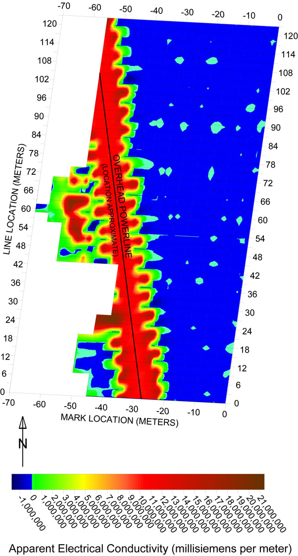
The anomalies in zone 1 appear to be located in a linear feature seen most clearly in the magnetic susceptibility as the red diagonal feature running south-southeast from about (35, 0) to (50, -45) (fig. 2B). Based on the EM and magnetic data, the anomalies tend to follow the ephemeral stream (fig. 4); however, the anomalies began to shift towards the east bank at line location -24 and became independent of the stream at line location -39 (figs. 2 and 3). Although the northern part of this anomaly zone could be attributed to the metal pipe and small arms waste located in the ephemeral stream (figs. 3 and 4), the anomaly in the east bank is more likely to be buried metallic objects. A visual investigation around the location where the anomalies began to shift towards the east bank revealed a piece of scrap metal in a small depression at (45,-30). In this area the vertical gradient data showed an elongated area of closely spaced high and low values, suggesting magnetization of metals in the subsurface. These anomalies were considered significant enough to be further investigated by 2D-DC resistivity.
The other major anomaly of AOC 3, located at (5, -33) and seen in both the magnetic susceptibility and vertical gradient datasets, could not be attributed to exposed surface waste (fig. 2B and C). Although this anomaly was much smaller in the EC results, a zone was designated around this anomaly based on the correlation between the magnetic susceptibility and vertical gradient results (fig. 3).
Figure 3. Site map of AOC 3 showing anomalous zones.
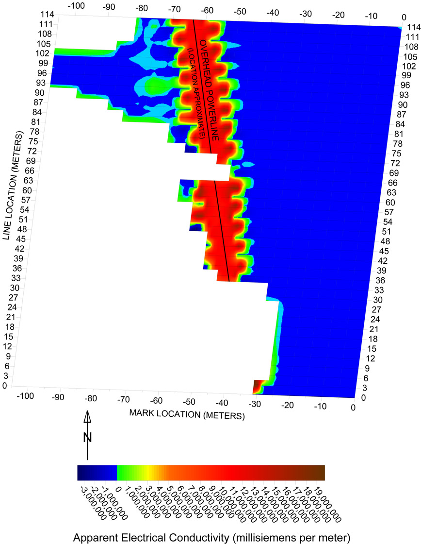
An overhead powerline runs roughly north-south in the western part of AOC 7 (fig. 8). Because the powerline oversaturates the GEM-2, the EM data surrounding the powerline must be ignored. To determine where the effect of the powerline was overpowering, the 60-Hz monitoring frequency was examined (fig. 5). The 60-Hz monitoring frequency shows a strong response in an area of approximately 10 meters on each side of the powerline. The total apparent EC shows a band in the same location, indicating the need to mask out this section of the AOC. Because of the effect of the powerline on the EM data, the magnetometer survey was given the most weight in identifying the anomalies, while the EM datasets were used for confirmation.
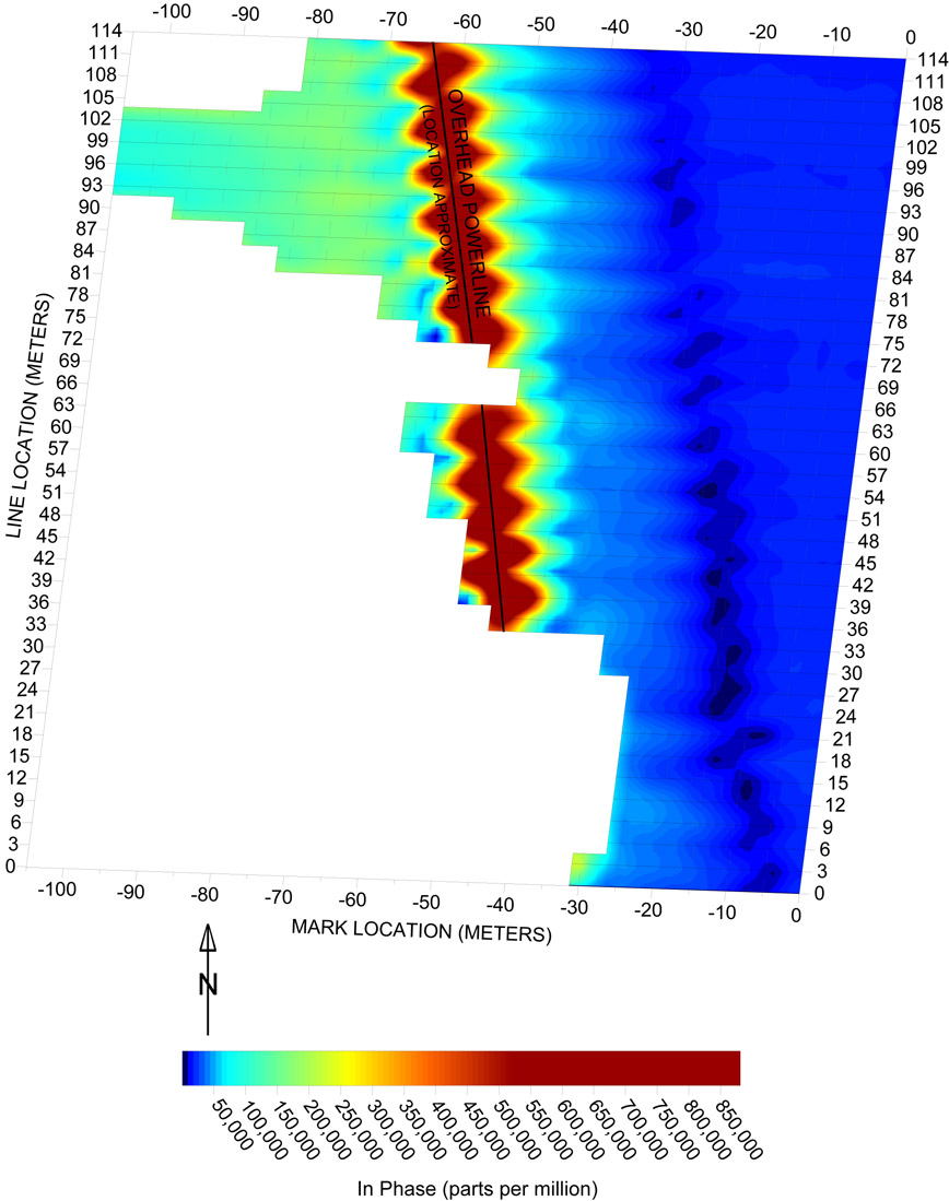
Anomalies in AOC 7 can be seen in the vertical gradient data that are not found to be major disturbances in the EM data (fig. 6). It should be noted that many of these vertical gradient features occur in the area influenced by the power lines where the EM method was compromised. Although large surface exposures of metallic debris were catalogued, smaller debris such as randomly distributed small arms waste, barbed wire, and other scrap metal may have been left undocumented under the dense vegetation throughout AOC 7. Such items could have caused the scattered features found in the vertical gradient data that were too small to be found with the EM method.
The largest anomaly occurred at (-40,117) to (-5, 90) (fig. 6). This feature appeared in both the magnetic susceptibility and the vertical gradient. This area was documented to have multiple metal sheets on the surface, as well as a large distribution of 1-inch diameter metal cable (fig. 7). Because of the high level of noise caused by the littering of surface metal, the EM and magnetic surveys were unable to determine if there was more waste buried at this location. Therefore, this anomaly was chosen for further investigation with 2D-DC resistivity (fig. 8).
Another relatively large anomaly appeared at (-5, 122), which was seen in all transmitted EM frequencies and magnetic data (fig. 6). At the surface a concrete "ring" was found, approximately 4 meters in diameter. Because of the strong response from both the EM and magnetic results, it was believed that metal also is present in the subsurface at this location, most likely as part of the structural support, such as rebar (fig. 8).
A somewhat linear anomaly running north-south ((-60, 72) to (–45, 48)) can be seen in all datasets (fig. 6). Although part of this zone falls within the powerline corridor (fig. 8), the correlation between the vertical gradient and magnetic susceptibility, in addition to the multiple surface exposures of small arms waste in this area (fig. 7B), caused these features to be delineated as a zone. Small arms waste is not expected to create a strong response in the vertical gradient, as the concentration of ferrous, or magnetic, materials is small in such debris. Because of the strong response shown in fig. 6B, it was suspected that more waste may be buried here in addition to the surface small arms waste. This anomaly was selected for further characterization by 2D-DC resistivity.
A small anomaly occurred in the magnetic susceptibility as well as the vertical gradient near (-20, 30) (fig. 6). No surface debris was recorded at this location. The clear response from both instruments validated creating a zone for this feature (fig. 8).
The magnetic susceptibility of 2,070 Hz shows a band of low intensity anomalies starting at (0, 39) and extending to (-20, 72) (fig. 6). However, the vertical gradient does not show similar anomalies within this area. Data collection in this area was impaired by heavy vegetation, steep topography, and vehicle traffic on the gravel road that borders AOC 7. Although there is the possibility that the anomaly found in the magnetic susceptibility was caused by subsurface metals, the difficulty experienced during data collection and the lack of corresponding anomalies in the vertical gradient results in a lower confidence level in delineating zone 7 than the other zones within AOC 7. However, the features seen in the magnetic susceptibility are strong enough to be classified as anomalies and are distributed over an area large enough to warrant creating a zone for these features.
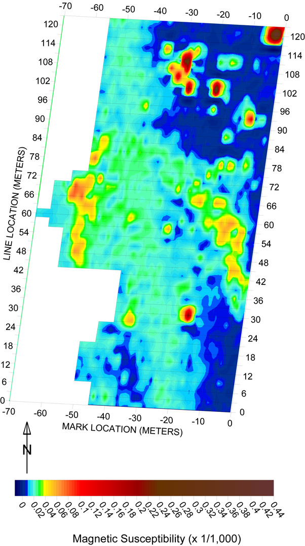
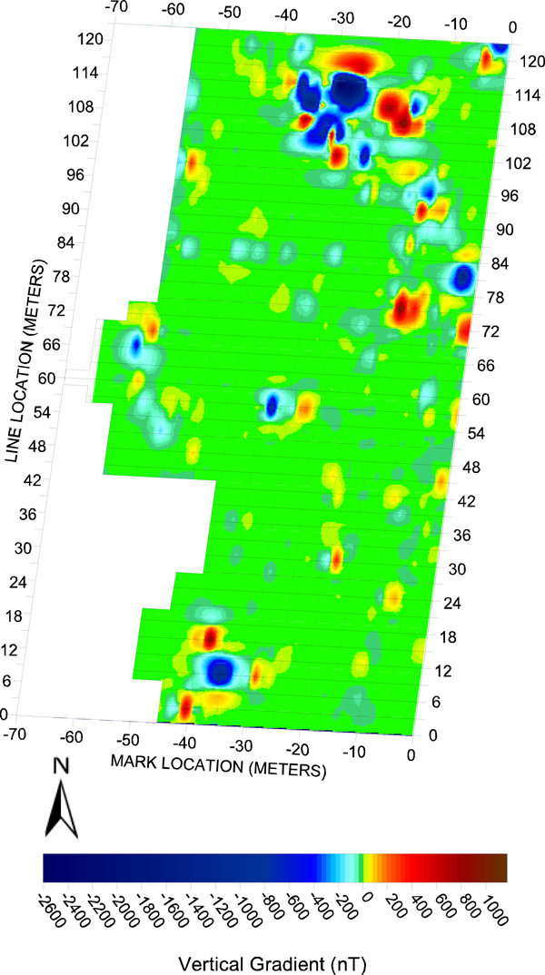
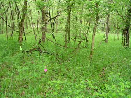
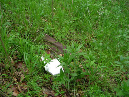
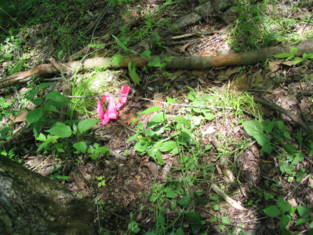
Figure 7-B1. B1 and B2, photographs of barbed wire and small arms waste near mark -55, line 51.
Figure 7-B2. B1 and B2, photographs of barbed wire and small arms waste near mark -55, line 51.
Figure 8. Site map of AOC 7 showing anomalous zones.
The overhead powerline running through AOC 7 continues into AOC 10, causing a similar oversaturation of the GEM-2 within the area of influence (fig. 5). Therefore, the vertical gradient data were determined to be the primary investigation technique, while the magnetic susceptibility was used as a secondary parameter. Like AOC 7, there was an abundance of scattered surface metal throughout AOC 10. Although large debris was recorded, not all surface metal could be located and documented by sight because of the vegetative cover. It is possible that the scattering of surface metal throughout AOC 10 caused the spotty high and low vertical gradient anomalies.
The most intense anomalies were found at (-80, 108) to (-70, 90) (fig. 9). This area was scattered with exposed steel drums, sheet metal, and other debris (fig. 10), which are the likely cause of these anomalies. The vertical gradient and magnetic susceptibility both showed more subtle anomalies extending 15 meters to the east. Though this area is within the powerline corridor, the agreement between the vertical gradient and magnetic susceptibility make it unlikely that these features are merely artifacts of electrical interference. These subtle features were grouped with the results of the exposed metal to create zone 8 (fig. 11).
The second major anomaly in the vertical gradient data was located near (-15, 30) (fig. 9). Scrap metal was catalogued on the surface at this location. However, the features shown in the vertical gradient and subtly in the magnetic susceptibility northward to line 42 may indicate additional buried ferrous metal. Another large anomaly at (-20, 51) did not correspond to a surface exposure. The correspondence between the vertical gradient and the magnetic susceptibility indicates that this location is likely to contain buried metal. Subtle magnetic susceptibility features surrounding these larger anomalies from line location 12 to 60 correspond to anomalies present in the vertical gradient. Because of the correlation, the area between (-10, 12) and (-20, 66) was grouped into zone 9.
Zones 10, 11 and 12 were created around small anomalies seen in both the magnetic susceptibility and the vertical gradient. Zone 10 is directly over the gravel road that runs along the eastern edge of AOC 10 and can be seen most clearly in the magnetic susceptibility at (0,102) (fig. 9). Despite the weaker response in the vertical gradient, the anomaly seen in the magnetic susceptibility warranted creating a small zone for this feature. Zones 11 and 12 were created around subtle features seen most clearly in the magnetic susceptibility at (-15, 75), and (-35, 111), respectively (fig. 9). Although these locations did not have a strong enough response in the EM method to qualify as an anomaly, the corresponding features in the vertical gradient indicate that metals could be present in the subsurface; therefore, a zone was created around each of these features.
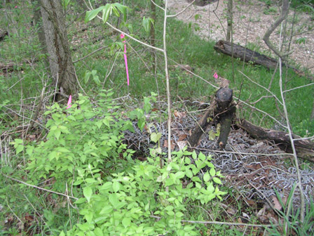
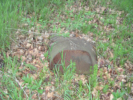
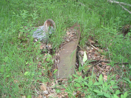
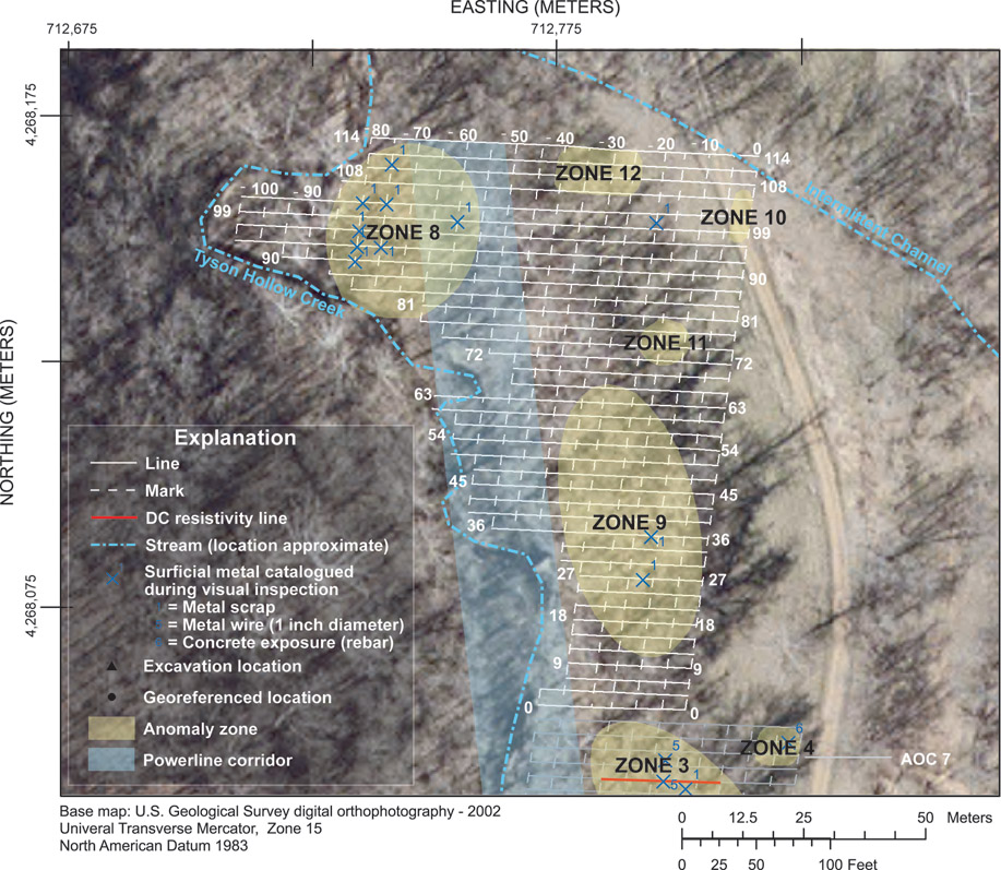
Figure 11. Site map of AOC 10 showing anomalous zones.
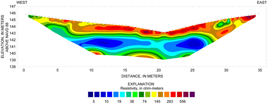
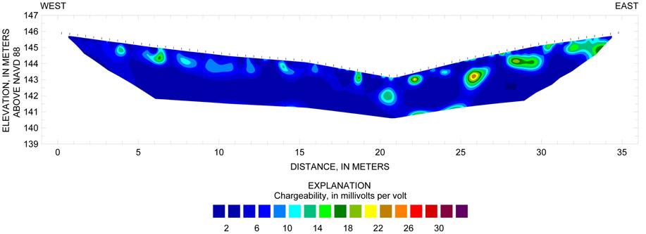
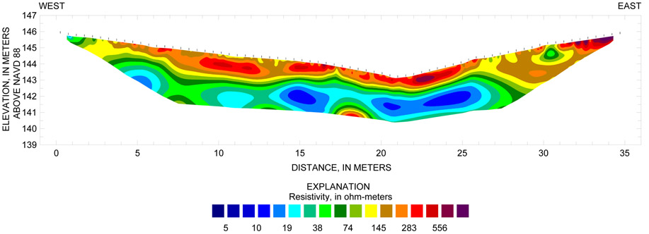
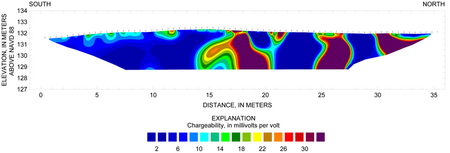
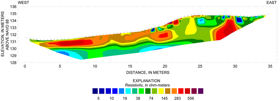
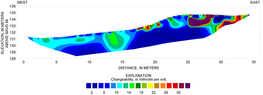
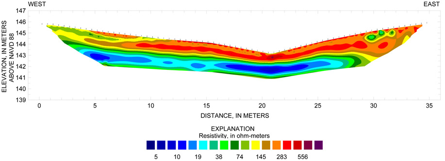
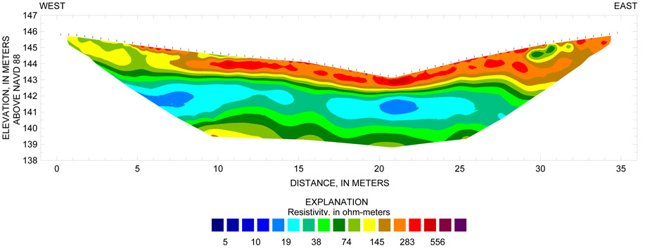
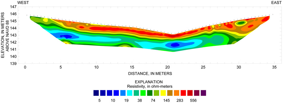
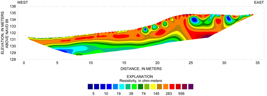
In addition to determining the areal extent of anomalies throughout each AOC, the vertical extents were determined for certain anomalies in AOCs 3 and 7. The vertical extents of selected anomalies were analyzed by examining the 2D-DC resistivity and time-domain IP data. The 2D-DC resistivity data were collected using a dipole-dipole and a Wenner-Schlumberger array for Line 1 (fig. 3). Time-domain IP measurements were also collected using the dipole-dipole array at survey line 1 (fig. 12A). The data from each array were inverted in the field and analyzed to determine the most effective array that would be used to collect data for additional survey lines. After reviewing the raw data and inversion results of the resistivity data, the Wenner-Schlumberger array (fig. 12B) was chosen for the collection of additional survey lines. Both the dipole-dipole and the Wenner-Schlumberger arrays produced similar results; however, due to the geometry of the array, the Wenner-Schlumberger array has a lower signal-to-noise ratio, producing the highest quality data for both the raw data and the inverted field resistivity datasets. The Wenner-Schlumberger array was subsequently used to collect 2D-DC resistivity and time-domain IP measurements for lines 2 through 5 (figs. 3 and 8). The results were displayed by plotting two-dimensional sections of the inverted field resistivity and inverted time-domain IP data in a gradational color scale (figs. 12, 13, 14, 15, and 16). The cooler colors are less resistive, or have a lower chargeability, and the warmer colors are more resistive, or have a higher chargeability. Inversion results of the resistivity data were displayed using a logarithmic scale and the time-domain IP inversion results are displayed using a linear scale of chargeability values.
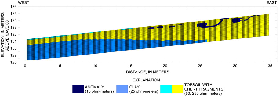
The inversion results of the field resistivity data from both the dipole-dipole and Wenner-Schlumberger arrays from survey line 1 (fig. 12) and the Wenner-Schlumberger array for survey lines 2 and 3 (figs. 13 and 14) were interpreted as having a similar 3-unit case whereas lines 4 and 5 (figs. 15 and 16) were more difficult to interpret because of the noise caused by surface and subsurface metallic debris. Line 4 was interpreted to have three resistivity units whereas line 5 was interpreted to have only two resistivity units. Unit 1 is a high resistivity unit (greater than 74 ohm-meters) followed by unit 2, a less resistive layer (less than 74 ohm-meters). Survey lines 1 through 3 also show a non-continuous high resistivity (greater than 74 ohm-meters) feature near the bottom of each section, which is considered to be unit 3. This unit was observed but its location was not clearly defined because of the reduction in sensitivity near the bottom of the section. Sensitivity represents the degree to which a change in the resistivity of a section of the subsurface will influence the potential measured by the array (Loke, 2000). Alterations in the location and properties of unit 3 in the model tend to have little effect on the inversion result because the bottom and edges of the section in a Wenner-Schlumberger array is the least sensitive part of the section. Because of this lower sensitivity, the contact surface of unit 3 is considered to be more poorly defined than other units. Areas within unit 1 that are less than 74 ohm-meters are considered to be anomalies and are found in survey lines 1, 2, 4, and 5 (figs. 12, 13, 15, and 16).
Sections of the inverted field chargeability data from time-domain IP measurements exhibit features throughout each section where chargeability increases more than 12 mV/V in comparison with the surrounding regions. These features are considered to be anomalies for survey lines 1 through 5 (figs.12, 13, 14, 15, and 16). Anomalies occurring within lines 1 though 5 are denoted by the display of colors representing 12mV/V or greater.
Time-domain IP measurements from survey lines 1, 2, and 3 showed a more frequent occurrence of anomalies than were shown in the field resistivity sections (figs. 12, 13, and 14). The lack of low resistivity anomalies shown in the resistivity sections of survey lines 1, 2 and 3 could possibly be explained by a relatively high concentration of highly resistive chert fragments in unit 1, as well as the scattered distribution of small arms waste throughout the soil matrix discovered during excavation activities. The chert could be acting as an insulator, masking the less-resistive inclusions of small arms waste. However, a charge could still be induced in the isolated small arms waste, causing a greater IP response than the surrounding topsoil and chert fragments.
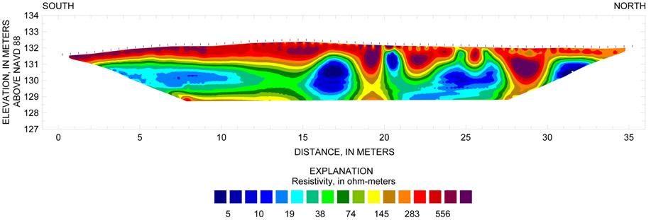
Survey lines 4 and 5 show large, low resistivity anomalies throughout the resistivity and time-domain IP sections (figs. 15 and 16). These low resistivity anomalies could be attributed to barbed wire (fig. 7B) found along survey line 4 and 1-inch diameter metal cable (fig. 7A) found along survey line 5. The presence of this surficial metal could have created preferential electrical conduits near the surface, causing the majority of the current transmitted by the current electrodes to reach the potential electrodes without traveling through the more resistive subsurface geology. The inversion process would have projected these low resistivity, surface-influenced readings at false depths, creating large, deep anomalies in the subsurface.
After the field data were examined, forward models were created for 2D-DC resistivity survey lines 1 through 5. The layers used in forward modeling were assigned resistivity values based on the field resistivity dataset and were altered according to the results of the model inversion. Geologic descriptions were given to each layer based on driller's logs: a resistivity of 250 ohm-meters was used to model the topsoil with chert fragments in layer 1, a resistivity of 25 ohm-meters was used to model the clay in layer 2, and a resistivity of 250 ohm-meters was used to model the limestone in layer 3. Layer 1 contains areas that range in resistivity, believed to result from variations in the abundance of chert fragments within the top soil. Therefore, some areas in layer 1 were modeled with values less than 250 ohm-meters. Values of 50 and 100 ohm-meters were used to represent areas of layer 1 where there was a decrease in resistivity. In survey line 3, layer 1 also contained areas where resistivity values increased (fig. 14). This area was located along an unnamed ephemeral stream (fig. 3) in AOC 3 and was associated with an increase in the abundance of gravel and cobble-sized chert, which was assigned a resistivity of 750 ohm-meters. Survey line 4 in AOC 7, near Tyson Hollow Creek (fig. 8), also had an increase in resistivity in layer 1 because of gravel- and cobble-sized chert. A value of 1,000 ohm-meters was used in layer 1 to indicate the area where resistivity increased, which is also considered to reflect an increase in the abundance of gravel- and cobble-sized chert deposits. Low resistivity anomalies in the inverted field resistivity data from survey lines 1, 2, and 5 were assigned a resistivity of 10 ohm-meters in the forward models for each line. Line 4 also contained low resistivity anomalies appearing in layer 1; however, to produce an inverted model resistivity section that closely corresponded with the inverted field resistivity data from line 4, a resistivity of 0.5 ohm-meter was used in the modeling of anomalies for survey line 4.
Line 1 forward model (fig. 17A) was used as the initial input model grid for lines 2 through 5. After many iterations, a three-layer model consisting of topsoil with chert fragments (layer 1), clay (layer 2), and limestone (layer 3) was produced for lines 1, 2, 3 and 4 (figs. 17A, 18A, 19A, and 20A). A two-layer model consisting of topsoil with chert fragments (layer 1) and clay (layer 2) was developed for survey line 5 in AOC 7 (fig. 21A). A model solution was reached when the inversion results of the model (figs. 17C, 18B, 19B, 20B, and 21B) visually resembled the inversion results from the field data (figs. 12B, 13A, 14A, 15A, 16A).
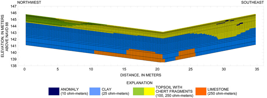
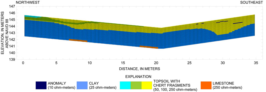
Interpretation sections were created for each survey line using results from both the field resistivity data and forward models. Lines 1 through 3 were interpreted primarily based on the field resistivity data, while forward models were used as a guideline for interpreting the field data. Because of the more complicated nature of the field resistivity data from survey lines 4 and 5, interpretations were based more heavily on the forward models than the field resistivity data, yielding a 3-layer interpretation for line 4 and a 2-layer interpretation for line 5. Because of the lower sensitivity of the bottom of the Wenner-Schlumberger array, the interpretation section does not accurately characterize the surface of layer 3 in any of the lines. Because of the remote nature of 2D-DC resistivity and the chance for variability in the subsurface, the interpretations are non-unique solutions to the field resistivity data (Degnan, 2001). Although it is possible to develop different interpretations that would also be reasonable solutions to the field resistivity data, the addition of information from driller's logs and excavation trenches makes the following interpreted sections likely scenarios.
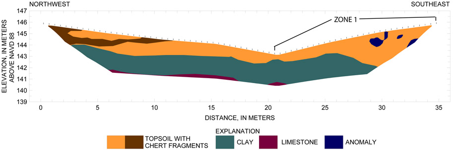
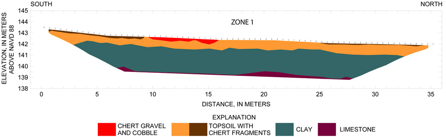
Layer 1 consists of topsoil with chert fragments occurring at land surface and ranging down to 144 to 142 meters (m) above the North American Vertical Datum of 1988 (NAVD 88). Clay is represented as layer 2, but the thickness of this layer could not be determined because no consistent third layer was found to define the lower boundary. Layer 3, limestone, is horizontally discontinuous. The contact between layers 2 and 3 occurs intermittently between 141 to 142 m in elevation in the northwestern part of the section and does not appear in the southeastern part of the section. Three anomalies were interpreted along the southeastern edge of the section in layer 1, extending below the surface to a depth of 1 to 1.5 m (fig. 22). This location corresponds to a strong anomaly seen clearly in both the magnetic susceptibility and vertical gradient at (50, -39) (fig. 2).
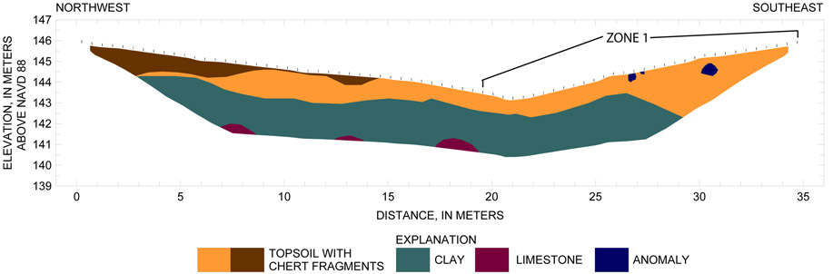
Layer 1, topsoil with chert fragments, occurs at the land surface and ranges down to 144.5 to 142.5 m in elevation. Layer 2 represents clay with an interpreted thickness between 1.5 and 2.5 m. Layer 3, composed of limestone, is divided into three sections that are located on the northwestern part of the line. There are three anomalies in layer 1 towards the southeastern edge of the section at depths of 0 to 1 m (fig. 23). The easternmost anomaly corresponds to the location of an anomaly in the magnetic susceptibility and total apparent electrical conductivity as well as the vertical gradient, near (50, -36) (fig. 2). The remaining two anomalies in the interpretation section are contained within the bounds of zone 1 (fig. 3).
Layer 1, topsoil with chert fragments, occurs in the upper 1 to 1.5 m of the section. The surface of layer 2, clay, was interpreted to be between 142.5 m elevation along the southern edge of the section and 141 m elevation along the northern edge of the section and to range in thickness from 2 to 2.5 m. Layer 3 represents limestone extending from the bottom of layer 2 to the bottom of the section. The surface of the limestone starts at about 140 m in elevation to the south and descends discontinuously to about 139 m elevation at the location distance of 27 m. No low resistivity anomalies were located in the inverted field resistivity (fig. 24).
The resistivity line crossed through surface exposures of small arms waste and barbed wire along the entire length of the line, which may have created a path for current flow generating large, low resistivity anomalies at greater depths than may be realistic. However, the forward model would be unable to predict this response caused by the surface debris, and therefore also reflects the deep anomalies that may be an artifact of surficial debris.
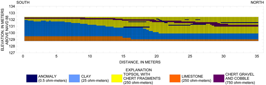
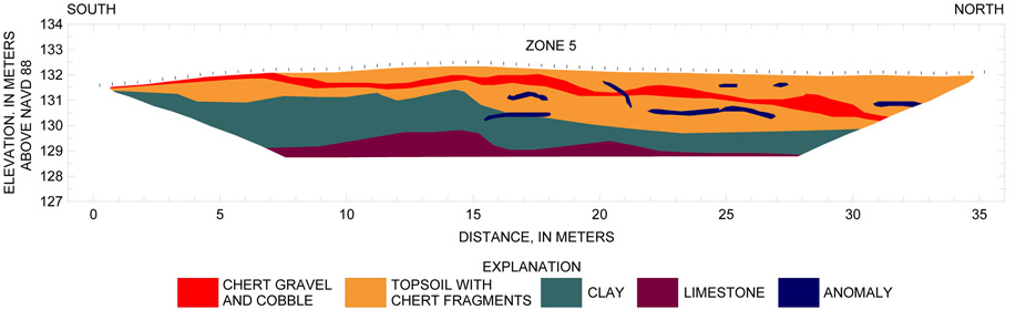
Topsoil and chert fragments (layer 1) were interpreted to be as thin as 0.5 m near the southern edge of the section and as thick as 2.5 m along the northern edge of the section. A layer of chert gravel and cobble, ranging from less than 0.25 m to about 1.0 meters thick, is interpreted to cut continuously through layer 1. Layer 2 (clay) ranges in elevation from about 131 m along the southern edge of the section to about 129 m at the northern edge of the section. Limestone (layer 3) ranges in elevation from about 128.5 m along the southern edge of the section to about 129.5 m at location distance 15 m then decreases in elevation to about 129 m at the southern edge of the section (fig. 25). Seven interpreted low resistivity anomalies of varying length occurred within layers 1 and 2, possibly resulting from the barbed wire found near the surface.
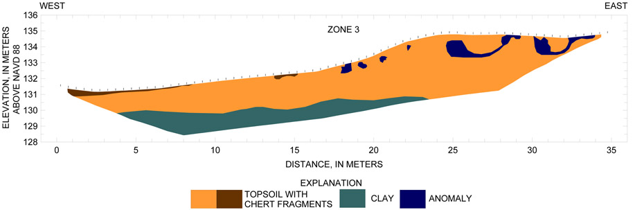
Layer 1, composed of topsoil with chert fragments, is found from an elevation of about 130 m to land surface. The second layer, interpreted to be clay, extends below the bottom of the section to an unknown depth. Several low resistivity anomalies were located in layer 1 of the inverted field resistivity data. These anomalies were modeled in layer 1 (topsoil with chert fragments) of the forward model for survey line 5. Forward modeling results were used to approximate the depth and size of these anomalies (fig. 26). The interpretation section of resistivity data from line 5 shows a scattering of low resistivity anomalies in the eastern part of the section to a depth of about 1.5 m below the surface. The time-domain IP data supports this depth and distribution. It is likely that the surficial waste extends into the subsurface about 1.5 m in zone 3 (fig. 8) at this location.
Excavation was performed at AOCs 3 and 7 to explore selected anomalies and suspicious surface debris and to assess the accuracy of the geophysical surveys. A total of nine locations were excavated during two events (trips) in AOCs 3 (E-1, E-2, E-3; fig. 3) and 7 (E-4 through E-8; fig. 8). Excavated soil was segregated by depth and placed on a tarp. Waste characterization was performed twice by the USACE, which consisted of filling a bucket with excavated soil and then determining the weight and volume of soil and small arms waste. A tractor-mounted backhoe was used to excavate the selected areas.
Trench 1 (E-1), oriented approximately east to west, (fig. 3) was completed to a depth of 0.6 m at AOC 3 near the east bank of the ephemeral stream. This location was chosen because of the scattering of small arms waste visible in the substrate of the stream channel. Small arms waste was found scattered throughout a brown silty clay soil matrix with chert fragments to a depth of approximately 0.3 m. A soil sample was collected at a depth of approximately 0.1 to 0.15 m, in the same zone as the small arms waste. The sample contained approximately 1 volumetric percent small arms waste. No anomalies were found in this location by any geophysical method used in this study, most likely because of the non- continuous scattering of a small quantity of metallic waste.
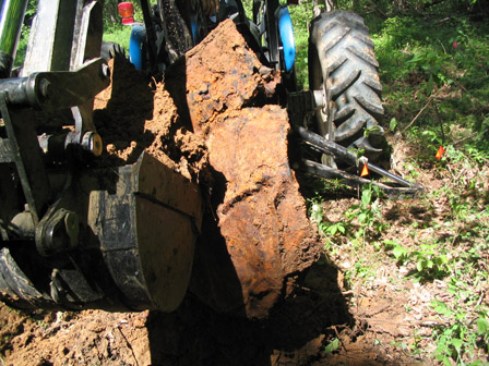
The second (E-2) and third (E-3) trenches were positioned to further investigate the southernmost anomaly found in zone 1 in the EM and magnetic results near (50, -42) (fig. 2), as well as in survey line 1 of the 2D-DC resistivity and time-domain surveys (fig. 12). E-2 (fig. 3) was excavated to about 1 m below land surface. No metallic debris was found at this location. After re-examination of the field data from the EM and magnetic surveys, excavation was repositioned to E-3. During excavation of E-3, a flattened 55-gallon drum was removed from approximately 0.3 m below land surface (fig. 27A). This drum was most likely the cause of the anomaly seen in figure 2.
Five trenches were completed at AOC 7. The first trench, E-4 (fig. 8), was approximately 0.8 m deep and opened generally in a west to east direction beginning in the streambed near the southwest corner of AOC 7 near grid location (-35, 12). A metal post was removed from the alluvium, which consisted of silt and chert fragments. Although vertical gradient data showed an anomaly at this location, the EM data did not show a similar feature. This discrepancy was likely caused by the powerline's influence over the GEM-2 within the powerline corridor, while the magnetometer was still able to successfully locate metallic debris.
The second trench, E-5 (fig. 8), was opened near grid location (-50, 81) in the east bank of Tyson Hollow Creek in a north to south direction and extended to a depth of approximately 0.3 m. This site was chosen because of a scattering of small arms waste on the surface and because grass had failed to grow at this location although the majority of the site was heavily vegetated. The EM and magnetic techniques did not show any anomalies in this location. The soil consisted of silty clay with chert fragments, and small arms waste appeared to extend to a depth of approximately 0.08 to 0.10 m. Although small arms waste was found at the surface, there was no indication that this deposit extended into the subsurface in high concentrations. Therefore, it is reasonable that no anomalies were found using these specific geophysical methods.
E-6, E-7, and E-8 were the third, fourth, and fifth trenches (fig. 8) and were east of the stream bank where small arms waste was exposed at the surface (fig. 7B) and EM, magnetic, 2D-DC resistivity, and time-domain IP data exhibited anomalies (figs. 6 and 15). E-6 was opened near grid location (-55, 51), generally in a west to east direction to a depth of approximately 0.9 m. Small arms waste appeared to extend to a depth of approximately 0.4 to 0.5 m. E-7 was excavated near grid location (-55, 69), generally in a north to south direction to a depth of approximately 0.6 m. Small arms waste was contained within the first 0.1 m. Barbed wire was located in the vicinity of E-6 and E-7 (fig. 7B). E-8 was excavated near grid location (-55, 54) to a depth of almost 1 m. Small arms waste (fig. 27B) was found within the upper 0.5 m in this trench.
The former Tyson Valley Powder Farm near Eureka, Missouri, was used primarily as a storage facility for the production of small arms ammunition at the nearby St. Louis Ordnance Plant during 1941–47 and 1951–61, although munitions testing and disposal took place on site as well. During U.S. Army activity at the site, shell casings, munitions, munitions components, storage drums, and miscellaneous metallic materials were disposed of throughout the property, remnants of which can still be seen on the surface and are believed to continue into the subsurface. However, little historical information exists describing disposal practices. Three areas of concern (AOC 3, AOC 7, and AOC 10), previously identified by the U.S. Army Corps of Engineers, were selected in spring 2004 for investigation by the U.S. Geological Survey, in cooperation with the U.S. Army Corps of Engineers, using four surface geophysical methods.
Electromagnetic and magnetic methods were used to determine the subsurface areal extent of metallic anomalies. Results from these methods were used to create maps identifying zones of anomalies within each of the areas of concern. Several zones were then selected for further investigation using two-dimensional direct-current resistivity and time-domain induced polarization (IP) methods to characterize the vertical extent of the anomalies in the selected zones. Using an inversion process, sections of the subsurface were developed from the data and were compared to anomaly locations from the electromagnetic and magnetic surveys. Excavations were made at selected locations to check the results of the four geophysical methods. The geophysical methods selected for use in this study were useful in determining the areal and vertical extent of metallic waste within the former Tyson Valley Powder Farm. However, electromagnetic and magnetic methods were not able to differentiate magnetic scrap metal from non-magnetic metallic small arms waste, most likely because of the small size and scattered distribution of the small arms waste, in addition to the mixing of both types of debris within the subsurface.
Electromagnetic and magnetic data showed a scattering of anomalies in all three areas of concern. Anomalous zones were identified and mapped—zones 1–2 in AOC 3, zones 3–7 in AOC 7, and zones 8–12 in AOC 10. Zones 1, 3, and 5 were selected for further investigation concerning the vertical extent of the anomalies.
In zone 1 (AOC 3), sections developed from the resistivity data along survey lines 1 and 2 indicated the presence of anomalies in layer 1 (topsoil with chert fragments). Sections from the time-domain IP measurements for survey lines 1, 2, and 3 showed a greater occurrence of anomalies in layer 1 and extending into layer 2. The lack of low resistivity anomalies shown in the resistivity section could possibly be explained by the high concentration of highly resistive chert fragments in layer 1. The chert could have been acting as an insulator, masking the less-resistive inclusions of small arms waste. However, once the small arms waste was "charged" using the time-domain IP method, it showed a greater response compared to the surrounding topsoil and chert fragments. Excavations showed buried scrap metal and scattered small arms waste in zone 1, and did not indicate the presence of any high-density continuous small arms waste deposits. Based on all of the results, anomalies in AOC 3 were believed to be a scattering of a variety of metallic waste that extends from the surface to a depth of approximately 1 meter, possibly as deep as 1.5 meters.
In zone 3 (AOC 7), resistivity line 5 crossed zone 3 through surface debris including 1-inch diameter metal cable and sheet metal. The field resistivity section for line 5 showed a scattering of low resistivity anomalies in the eastern part of the section to a depth of approximately 1.5 meters below the surface. The time-domain IP section confirmed this depth and distribution. Visual reconnaissance showed the metal cable entering the ground in multiple locations. The scattered surface metal likely extends into the ground to a depth of approximately 1.5 meters, possibly to 2 meters, below the surface.
Zone 5 (AOC 7) was bisected lengthwise by resistivity line 4 and crossed through multiple surface exposures of shell casings and barbed wire. The resistivity section showed anomalies extending to a maximum of 1.5 meters below the surface. Excavations along the resistivity line showed small arms waste present in the soil to an approximate depth of 0.5 meter below the land surface, although the interpretation of resistivity data indicates anomalies extend to a greater depth. Barbed wire along the survey line may have created a path for current flow, causing low resistivity anomalies to extend below their actual depths.
Benham, K.E., 1982, Soil survey of St. Louis County and St. Louis City, Missouri: Washington, D.C., U.S. Department of Agriculture—Soil Conservation Service: U.S. Government Printing Office, Washington, DC.
Breiner, Sheldon, 1999, Applications manual for portable magnetometers: San Jose, California, Geometrics, accessed April 2004 at URL http://www.geometrics.com/
Criss, R.E., 2001, Hydrogeology of Tyson Research Center, Lone Elk County Park, and West Tyson County Park, eastern Missouri, Tyson Valley (ex) Army Powder Storage Farm site file: U.S. Environmental Protection Agency, Region 7, 58 p.; also at http://www.biology.wustl.edu/tyson/geology.html (accessed April 2004).
Degnan, J.R., Moore, R.B., and Mack, T.J., 2001, Geophysical investigations of well fields to characterize fractured-bedrock aquifers in southern New Hampshire: U.S. Geological Survey Water-Resources Investigations Report 01-4183, 54 p.
Ellis Environmental Group, 2003, Draft Phase I, II, III Remedial investigation and risk assessment report, former Tyson Valley Powder Farm, Eureka, Missouri: Newberry, Florida, Prepared for the U.S. Army Corps of Engineers by Ellis Environmental Group, September 2003.
Geometrics, 2004, G-858 magnetometer flyer: San Jose, California, Geometrics, accessed May 2004 at URL http://www.geometrics.com/
Geophex, Ltd., 2004, GEM-2 flyer: Raleigh, North Carolina, Geophex, Ltd., accessed May 2004 at URL http://www.geophex.com/
Huang, H., and Won, I.J., 2000, Conductivity and susceptibility mapping using broadband electromagnetic sensors: Journal of Environmental and Engineering Geophysics, v. 5, no. 4, p. 31-41.
HydroGeoLogic, 1999, Final data summary report, Phase II remedial investigation, Tyson Valley Powder Farm, Eureka, Missouri: Overland, Kansas, HydroGeoLogic, Inc., March 1999.
Kring, Debbie, and Bailey, D., 2001, Tyson Valley (ex.) Army Powder Storage Farm, St. Louis, Missouri: U.S. Environmental Protection Agency Region 7 Fact Sheet, 2 p.
Loke, M.H., 2000, Electrical imaging surveys for environmental and engineering studies—a practical guide to 2D and 3D surveys: Penang, Malaysia, M.H. Loke, accessed September 2000 at URL http://www.agiusa.com/literature.shtml
Loke, M.H., 2002, RES2DMOD version 3.01—Rapid 2D resistivity forward modeling using the finite-difference and finite element methods: accessed October 1, 2003, at URL http://www.geoelectrical.com
Loke, M.H., 2003, RES2DINV version 3.52w—Rapid 2D resistivity and IP inversion using the least-squares method: Geoelectrical Imaging 2-D and 3-D—Geotomo Software, 125 p., accessed August 10, 2003, at URL http://www.geoelectrical.com
Loke, M.H., 2004, Tutorial—2-D and 3-D electrical imaging surveys: Geotomo Software, 12 p., accessed July 23, 2004, at URL http://www.geoelectrical.com
Natural Resource Conservation Service, 2004, Official soil descriptions: accessed May 17, 2004 at URL http://soils.usda.gov/technical/classification/osd/
Powers, C.J., Wilson, Joanna, Haeni, F.P., and Johnson, C.D., 1999, Surface-geophysical characterization of the University of Connecticut landfill, Storrs, Connecticut: U.S. Geological Survey Water-Resources Investigations Report 99-4211, 34 p.
Stanton, G.P., Kress, W.H., Hobza, C.M., and Czarneci, J.B., 2003, Possible extent and depth of salt contamination in ground water using geophysical techniques, Red River aluminum site, Stamps, Arkansas, April 2003: U.S. Geological Survey Water-Resources Investigations Report 03-4292, p. 5-19.
U.S. Army Corps of Engineers, 2001, Scope of work for .30- and .50-caliber shell casing disposal, AOC 3, Former Tyson Valley Powder Farm: U.S. Army Corps of Engineers, Kansas City District, 8 May 2001.
Won, I.J., 2003, Small frequency-domain electromagnetic induction sensor—How in the world does a small broadband EMI sensor with little or no source-receiver separation work?: The Leading Edge, April issue, p. 320-322.
Won, I.J., and Keiswetter, D.A., 1997, Comparison of magnetic and electromagnetic data for underground structures: Journal of Environmental and Engineering Geophysics: v. 2, no. 2, p. 115-126.
Won, I.J., Keiswetter, D.A., Fields, G.R.A, and Sutton, L.C., 1996, GEM-2—A new multifrequency electromagnetic sensor: Journal of Environmental and Engineering Geophysics, v. 1, no. 2, 129-138 p.
Table 1-1. Georeferenced locations within AOC 3.
[All units are in meters; Coordinate System: Universal Transverse Mercater Zone 15, North American Datum of 1983, elevation is in meters above the North American Vertical Datum of 1988; N/A, not applicable]
| Line Location | Mark Location | Northing | Easting | Elevation | Point Description |
|---|---|---|---|---|---|
| -3 | 0 | 4268411.411 | 713528.494 | 148.4161 | Grid point |
| -3 | 50 | 4268390.604 | 713572.594 | 143.2731 | Grid point |
| -6 | 0 | 4268408.512 | 713528.3998 | 148.4859 | Grid point |
| -6 | 50 | 4268387.45 | 713572.3893 | 143.4366 | Grid point |
| -9 | 0 | 4268405.665 | 713528.0822 | 148.8196 | Grid point |
| -9 | 50 | 4268384.548 | 713572.0385 | 143.5966 | Grid point |
| -9 | 50 | 4268384.371 | 713572.008 | 143.6951 | Grid point |
| -12 | 0 | 4268402.793 | 713527.7922 | 149.0879 | Grid point |
| -12 | 45 | 4268383.553 | 713566.8536 | 143.343 | Grid point |
| -12 | 50 | 4268381.361 | 713571.5122 | 143.7705 | Grid point |
| -15 | 0 | 4268399.895 | 713527.6211 | 149.4011 | Grid point |
| -15 | 45 | 4268380.56 | 713566.238 | 145.263 | Grid point |
| -15 | 50 | 4268378.161 | 713570.9369 | 143.9991 | Grid point |
| -18 | 0 | 4268397.395 | 713527.5124 | 149.9289 | Grid point |
| -18 | 45 | 4268377.685 | 713566.0703 | 143.8356 | Grid point |
| -18 | 45 | 4268377.665 | 713566.0809 | 143.8836 | Grid point |
| -18 | 50 | 4268374.814 | 713570.7857 | 144.2181 | Grid point |
| -21 | 0 | 4268395.016 | 713527.1923 | 150.2409 | Grid point |
| -21 | 45 | 4268374.495 | 713565.5861 | 144.011 | Grid point |
| -21 | 50 | 4268372.08 | 713570.0079 | 144.2701 | Grid point |
| -24 | 0 | 4268391.641 | 713526.7689 | 150.3229 | Grid point |
| -24 | 50 | 4268369.602 | 713569.6751 | 144.3631 | Grid point |
| -27 | 0 | 4268388.601 | 713526.5006 | 150.3344 | Grid point |
| -27 | 50 | 4268365.958 | 713569.3766 | 144.6166 | Grid point |
| -30 | 0 | 4268385.615 | 713526.1987 | 150.2949 | Grid point |
| -30 | 50 | 4268363.21 | 713569.1842 | 144.8636 | Grid point |
| -33 | 0 | 4268382.923 | 713525.9751 | 150.3119 | Grid point |
| -33 | 50 | 4268360.027 | 713568.8431 | 144.9671 | Grid point |
| -36 | 0 | 4268379.637 | 713525.6574 | 150.3314 | Grid point |
| -36 | 50 | 4268358.04 | 713567.8629 | 145.0996 | Grid point |
| -39 | 0 | 4268376.6 | 713525.3768 | 150.3339 | Grid point |
| -42 | 0 | 4268373.677 | 713524.9511 | 150.1584 | Grid point |
| -45 | 0 | 4268370.824 | 713524.8305 | 150.2249 | Grid point |
| -48 | 0 | 4268367.634 | 713524.561 | 150.4749 | Grid point |
| N/A | N/A | 4268401.216 | 713570.7704 | 142.8616 | Monitoring Well: MW3 |
| N/A | N/A | 4268395.697 | 713521.4441 | 150.6224 | Northwest corner of the Popping Kettle building |
| N/A | N/A | 4268395.16 | 713570.5174 | 143.0901 | Yellow benchmark disk: RANDAPLS2579 |
Table 1-2. Georeferenced locations within AOC 7.
[All units are in meters; Coordinate System: Universal Transverse Mercater Zone 15, North American Datum of 1983, elevation is in meters above the North American Vertical Datum of 1988; N/A, not applicable]
| Mark Location | Line Location | Northing | Easting | Elevation | Point Description |
|---|---|---|---|---|---|
| 0 | 0 | 4267928.137 | 712809.2012 | 135.95 | Grid point |
| 0 | -25 | 4267929.988 | 712784.4486 | 134.38 | Grid point |
| 0 | -25 | 4267929.965 | 712784.764 | 134.36 | Grid point |
| 3 | 0 | 4267932.789 | 712808.7444 | 133.88 | Grid point |
| 3 | -25 | 4267932.849 | 712784.8756 | 134.42 | Grid point |
| 6 | 0 | 4267935.804 | 712809.295 | 133.71 | Grid point |
| 6 | -25 | 4267935.908 | 712785.3969 | 134.52 | Grid point |
| 9 | 0 | 4267936.653 | 712810.5884 | 135.29 | Grid point |
| 9 | 0 | 4268061.566 | 712803.2501 | 134.42 | Grid point |
| 9 | -25 | 4267938.81 | 712785.8075 | 134.42 | Grid point |
| 12 | 0 | 4267939.601 | 712811.0294 | 134.99 | Grid point |
| 12 | -30 | 4267942.002 | 712781.357 | 133.46 | Grid point |
| 15 | 0 | 4267942.792 | 712811.4596 | 135.11 | Grid point |
| 15 | -30 | 4267945.147 | 712781.7472 | 133.30 | Grid point |
| 18 | 0 | 4267945.728 | 712811.8017 | 134.90 | Grid point |
| 18 | -30 | 4267948.131 | 712782.1512 | 133.16 | Grid point |
| 21 | 0 | 4267948.657 | 712812.2523 | 134.66 | Grid point |
| 21 | -30 | 4267950.94 | 712782.6141 | 133.05 | Grid point |
| 24 | 0 | 4267951.648 | 712812.7039 | 134.43 | Grid point |
| 24 | -30 | 4267954.042 | 712783.0265 | 133.01 | Grid point |
| 27 | 0 | 4267954.658 | 712813.0066 | 134.38 | Grid point |
| 27 | -35 | 4267957.195 | 712778.4306 | 132.48 | Grid point |
| 30 | 0 | 4267957.627 | 712813.4741 | 134.37 | Grid point |
| 30 | -35 | 4267960.497 | 712778.7926 | 132.45 | Grid point |
| 33 | 0 | 4267960.612 | 712813.8225 | 134.43 | Grid point |
| 33 | -35 | 4267963.107 | 712779.0301 | 132.32 | Grid point |
| 36 | 0 | 4267963.598 | 712814.2095 | 134.38 | Grid point |
| 36 | -40 | 4267966.208 | 712774.7161 | 132.35 | Grid point |
| 39 | 0 | 4267966.37 | 712814.5616 | 134.34 | Grid point |
| 39 | -40 | 4267969.336 | 712774.8814 | 132.31 | Grid point |
| 42 | 0 | 4267969.572 | 712814.9288 | 134.29 | Grid point |
| 42 | -40 | 4267972.52 | 712775.316 | 132.13 | Grid point |
| 45 | 0 | 4267972.965 | 712815.3445 | 134.83 | Grid point |
| 45 | -40 | 4267975.205 | 712775.7193 | 132.17 | Grid point |
| 48 | -40 | 4267978.272 | 712776.4123 | 132.53 | Grid point |
| 51 | -40 | 4267980.428 | 712776.7662 | 132.67 | Grid point |
| 54 | 0 | 4267980.992 | 712816.8908 | 135.00 | Grid point |
| 54 | -45 | 4267983.524 | 712772.6194 | 132.67 | Grid point |
| 57 | -45 | 4267986.666 | 712772.9462 | 132.54 | Grid point |
| 60 | -45 | 4267990.015 | 712773.4244 | 132.29 | Grid point |
| 63 | -45 | 4267992.336 | 712773.8831 | 132.02 | Grid point |
| 66 | -45 | 4267995.254 | 712774.3551 | 131.80 | Grid point |
| 69 | -45 | 4267998.001 | 712774.6861 | 131.58 | Grid point |
| 72 | -45 | 4268001.03 | 712775.3072 | 131.86 | Grid point |
| 111 | 0 | 4268037.658 | 712824.3585 | 134.96 | Grid point |
| 114 | 0 | 4268040.628 | 712824.7071 | 134.83 | Grid point |
| 114 | 0 | 4268040.892 | 712824.746 | 134.86 | Grid point |
| 114 | -5 | 4268040.956 | 712819.9719 | 134.79 | Grid point |
| 117 | 0 | 4268043.589 | 712825.2137 | 134.76 | Grid point |
| 117 | -5 | 4268043.628 | 712820.2921 | 134.76 | Grid point |
| 120 | 0 | 4268046.475 | 712825.5124 | 134.75 | Grid point |
| 120 | -5 | 4268046.532 | 712820.7092 | 134.93 | Grid point |
| 123 | 0 | 4268049.451 | 712826.0076 | 134.75 | Grid point |
| 123 | -5 | 4268049.645 | 712821.0606 | 134.80 | Grid point |
| 123 | -40 | 4268050.684 | 712786.2554 | 132.70 | Grid point |
| N/A | N/A | 4267890.814 | 712786.2602 | 135.07 | Power pole: PP364779 |
| N/A | N/A | 4267923.064 | 712829.4296 | 136.50 | Power pole: PP364780 |
| N/A | N/A | 4267942.26 | 712782.726 | 133.49 | Power pole: PP364790 |
Table 1-3. Georeferenced locations within AOC10.
[All units are in meters; Coordinate System: Universal Transverse Mercater Zone 15, North American Datum of 1983, elevation is in meters above the North American Vertical Datum of 1988; N/A, not applicable]
| Line Location | Mark Location | Northing | Easting | Elevation | Point Description |
|---|---|---|---|---|---|
| 0 | 0 | 4268052.919 | 712801.9002 | 134.54 | Grid point |
| 0 | -15 | 4268053.402 | 712787.1048 | 133.65 | Grid point |
| 9 | 0 | 4268061.64 | 712803.2616 | 134.42 | Grid point |
| 9 | -20 | 4268062.441 | 712783.741 | 132.53 | Grid point |
| 27 | 0 | 4268079.493 | 712805.8849 | 134.15 | Grid point |
| 36 | 0 | 4268088.361 | 712807.1011 | 134.10 | Grid point |
| 42 | 0 | 4268094.338 | 712807.6285 | 133.90 | Grid point |
| 45 | 0 | 4268097.325 | 712807.942 | 133.73 | Grid point |
| 48 | 0 | 4268100.268 | 712808.3141 | 133.67 | Grid point |
| 51 | 0 | 4268103.282 | 712808.6508 | 133.61 | Grid point |
| 54 | 0 | 4268106.277 | 712809.0405 | 133.70 | Grid point |
| 54 | -5 | 4268106.699 | 712804.142 | 133.64 | Grid point |
| 57 | 0 | 4268109.198 | 712809.3741 | 133.73 | Grid point |
| 57 | -5 | 4268109.636 | 712804.4055 | 133.74 | Grid point |
| 60 | 0 | 4268112.174 | 712809.7435 | 133.65 | Grid point |
| 60 | -5 | 4268112.489 | 712804.8566 | 133.70 | Grid point |
| 63 | 0 | 4268115.12 | 712810.134 | 133.65 | Grid point |
| 63 | -10 | 4268115.486 | 712800.2782 | 133.70 | Grid point |
| 66 | 0 | 4268118.116 | 712810.4866 | 133.64 | Grid point |
| 66 | -15 | 4268118.839 | 712795.6781 | 133.69 | Grid point |
| 69 | 0 | 4268121.182 | 712810.9077 | 133.54 | Grid point |
| 69 | -15 | 4268121.83 | 712796.1919 | 133.61 | Grid point |
| 72 | 0 | 4268124.062 | 712811.3565 | 133.51 | Grid point |
| 72 | -15 | 4268124.829 | 712796.5147 | 133.43 | Grid point |
| 75 | 0 | 4268127.052 | 712811.7302 | 133.45 | Grid point |
| 75 | -15 | 4268127.731 | 712796.8367 | 133.36 | Grid point |
| 78 | 0 | 4268130.043 | 712812.2016 | 133.47 | Grid point |
| 78 | -20 | 4268130.996 | 712792.4007 | 133.36 | Grid point |
| 81 | 0 | 4268132.94 | 712812.5533 | 133.49 | Grid point |
| 81 | 0 | 4268132.976 | 712812.6697 | 133.47 | Grid point |
| 81 | -25 | 4268134.265 | 712787.7501 | 133.48 | Grid point |
| 84 | 0 | 4268135.926 | 712812.9699 | 133.53 | Grid point |
| 84 | -25 | 4268137.166 | 712788.1385 | 133.45 | Grid point |
| 87 | 0 | 4268138.955 | 712813.4883 | 133.57 | Grid point |
| 87 | -25 | 4268140.127 | 712788.6337 | 133.39 | Grid point |
| 90 | -25 | 4268143.117 | 712788.9688 | 133.39 | Grid point |
| 93 | -25 | 4268146.107 | 712789.3261 | 133.41 | Grid point |
| 96 | -30 | 4268149.417 | 712784.7857 | 133.33 | Grid point |
| 99 | -35 | 4268152.599 | 712780.102 | 133.27 | Grid point |
| 102 | -35 | 4268155.528 | 712780.4485 | 133.30 | Grid point |
| 105 | -35 | 4268159.628 | 712780.9841 | 133.32 | Grid point |
| 108 | -35 | 4268162.788 | 712781.5416 | 133.39 | Grid point |
| 111 | -25 | 4268164.785 | 712791.7136 | 133.16 | Grid point |
| 111 | -35 | 4268165.39 | 712781.7606 | 133.38 | Grid point |
| 114 | -30 | 4268168.19 | 712787.1629 | 133.28 | Grid point |
| 114 | -40 | 4268169.024 | 712777.2493 | 133.08 | Grid point |
[All units are in meters; Coordinate System: Universal Transverse Mercator Zone 15, North American Datum of 1983]
| Zone | Easting | Northing |
|---|---|---|
| 1 | 713562 | 4268350 |
| 1 | 713572 | 4268350 |
| 1 | 713574 | 4268360 |
| 1 | 713566 | 4268400 |
| 1 | 713553 | 4268400 |
| 2 | 713528 | 4268380 |
| 2 | 713535 | 4268390 |
| 2 | 713536 | 4268380 |
| 2 | 713529 | 4268390 |
| 3 | 712817 | 4268000 |
| 3 | 712806 | 4268000 |
| 3 | 712799 | 4268020 |
| 3 | 712787 | 4268030 |
| 3 | 712783 | 4268050 |
| 3 | 712791 | 4268050 |
| 3 | 712812 | 4268040 |
| 3 | 712822 | 4268020 |
| 4 | 712824 | 4268040 |
| 4 | 712818 | 4268040 |
| 4 | 712818 | 4268050 |
| 4 | 712825 | 4268050 |
| 5 | 712766 | 4267980 |
| 5 | 712760 | 4267980 |
| 5 | 712769 | 4268020 |
| 5 | 712771 | 4268000 |
| 5 | 712761 | 4268000 |
| 6 | 712796 | 4267960 |
| 6 | 712800 | 4267960 |
| 6 | 712795 | 4267960 |
| 6 | 712792 | 4267960 |
| 7 | 712808 | 4267970 |
| 7 | 712805 | 4267980 |
| 7 | 712796 | 4267990 |
| 7 | 712797 | 4268000 |
| 7 | 712807 | 4268000 |
| 7 | 712817 | 4267990 |
| 7 | 712815 | 4267970 |
| 8 | 712730 | 4268140 |
| 8 | 712728 | 4268150 |
| 8 | 712746 | 4268170 |
| 8 | 712760 | 4268150 |
| 8 | 712747 | 4268130 |
| 9 | 712796 | 4268060 |
| 9 | 712805 | 4268080 |
| 9 | 712803 | 4268100 |
| 9 | 712786 | 4268120 |
| 9 | 712776 | 4268100 |
| 9 | 712780 | 4268080 |
| 10 | 712798 | 4268120 |
| 10 | 712803 | 4268130 |
| 10 | 712799 | 4268130 |
| 10 | 712792 | 4268130 |
| 11 | 712812 | 4268150 |
| 11 | 712814 | 4268160 |
| 11 | 712811 | 4268150 |
| 11 | 712815 | 4268150 |
| 12 | 712791 | 4268160 |
| 12 | 712776 | 4268160 |
| 12 | 712778 | 4268170 |
| 12 | 712792 | 4268170 |
Document Accessibility: Adobe Systems Incorporated has information about PDFs and the visually impaired. This information provides tools to help make PDF files accessible. These tools convert Adobe PDF documents into HTML or ASCII text, which then can be read by a number of common screen-reading programs that synthesize text as audible speech. In addition, an accessible version of Acrobat Reader 6.0, which contains support for screen readers, is available. These tools and the accessible reader may be obtained free from Adobe at Adobe Access.
| AccessibilityFOIAPrivacyPolicies and Notices | |
 |
|